Stochastic Wasserstein Singular Vectors
This Jupyter Notebook will walk you through an easy example of stochastic computation of Wasserstein Singular Vectors. This example is small enough to be run on CPU.
Imports
[1]:
import wsingular
import torch
import matplotlib.pyplot as plt
<frozen importlib._bootstrap>:219: RuntimeWarning: scipy._lib.messagestream.MessageStream size changed, may indicate binary incompatibility. Expected 56 from C header, got 64 from PyObject
Generate toy data
[2]:
# Define the dtype and device to work with.
dtype = torch.double
device = "cpu"
[3]:
# Define the dimensions of our problem.
n_samples = 20
n_features = 30
[4]:
# Initialize an empty dataset.
dataset = torch.zeros((n_samples, n_features), dtype=dtype)

# Iterate over the features and samples.
for i in range(n_samples):
    for j in range(n_features):

        # Fill the dataset with translated histograms.
        dataset[i, j] = i/n_samples - j/n_features
        dataset[i, j] = torch.abs(dataset[i, j] % 1)

# Take the distance to 0 on the torus.
dataset = torch.min(dataset, 1 - dataset)

# Make it a guassian.
dataset = torch.exp(-(dataset**2) / 0.1)
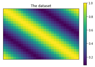
[5]:
# Plot the dataset.
plt.title('The dataset')
plt.imshow(dataset)
plt.colorbar()
plt.xticks([])
plt.yticks([])
plt.show()
Compute the WSV
[6]:
# Compute the WSV.
C, D = wsingular.stochastic_wasserstein_singular_vectors(
    dataset,
    dtype=dtype,
    device=device,
    n_iter=1_000,
    sample_prop=1e-1,
)
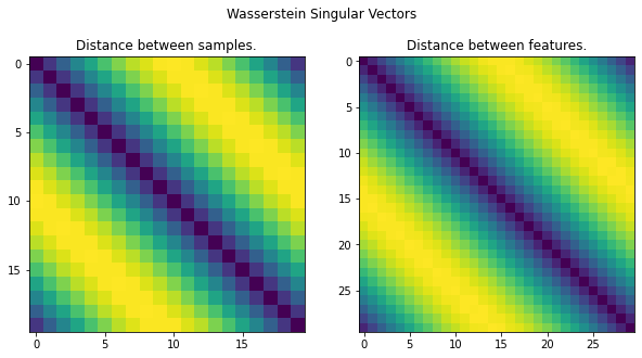
[7]:
# Display the WSV.
fig, axes = plt.subplots(1, 2, figsize=(10, 5))
fig.suptitle('Wasserstein Singular Vectors')

axes[0].set_title('Distance between samples.')
axes[0].imshow(D)
axes[0].set_xticks(range(0, n_samples, 5))
axes[0].set_yticks(range(0, n_samples, 5))

axes[1].set_title('Distance between features.')
axes[1].imshow(C)
axes[1].set_xticks(range(0, n_features, 5))
axes[1].set_yticks(range(0, n_features, 5))

plt.show()
[8]:
A, B = wsingular.utils.normalize_dataset(dataset, dtype=dtype, device=device)
wsingular.utils.check_uniqueness(A, B, C, D)
[8]:
True